DSP -> radio

from RF chaos to tuning in to the local broadcast

Imagine listening to the radio in your car and wondering, "hmm, i wonder how that works?". after a couple hours and another rabbit hole, you have in front of your a Raspberry Pi, an RTL-SDR dongle, and a mess of antennas. before this you didn't even know what GQRX was, and now you're trying to implement the backend from scratch. soon, your find yourself in the physics stack exchange re-teaching yourself E&M concepts from Physics II. and then, you have the epiphany, "i think i can demodulate the signal myself"
... from scratch.

Project planning — project planning and research (pure joy after we figured out all the EM-physics).

why build apollo?

We already had GQRX doing perfect FM playback, so why re‑implement it?

The motivation was basically:
- Treat the RTL‑SDR v2 (RTL2832 + FC0013) as a front‑end that gives us complex baseband samples.
- Design a full digital signal processing (DSP) chain ourselves: channel filtering, FM demod, de‑emphasis, decimation, resampling, AGC.
- Prove that it works both offline and real‑time, including on constrained hardware like a Raspberry Pi.

On the hardware side, the setup was:
- Raspberry Pi 3B (64‑bit Raspbian)
- RTL‑SDR v2 USB stick
- Stock telescopic antenna + an upgraded DAB/FM antenna (PAL → SMA)

The Pi could capture at 2.048MS/s, but doing everything (capture + DSP + audio out) on it pushed the CPU pretty hard. So the workflow ended up being: Pi for acquisition and real‑time experiments, laptops (Linux/Windows) for cleaner playback and debugging.

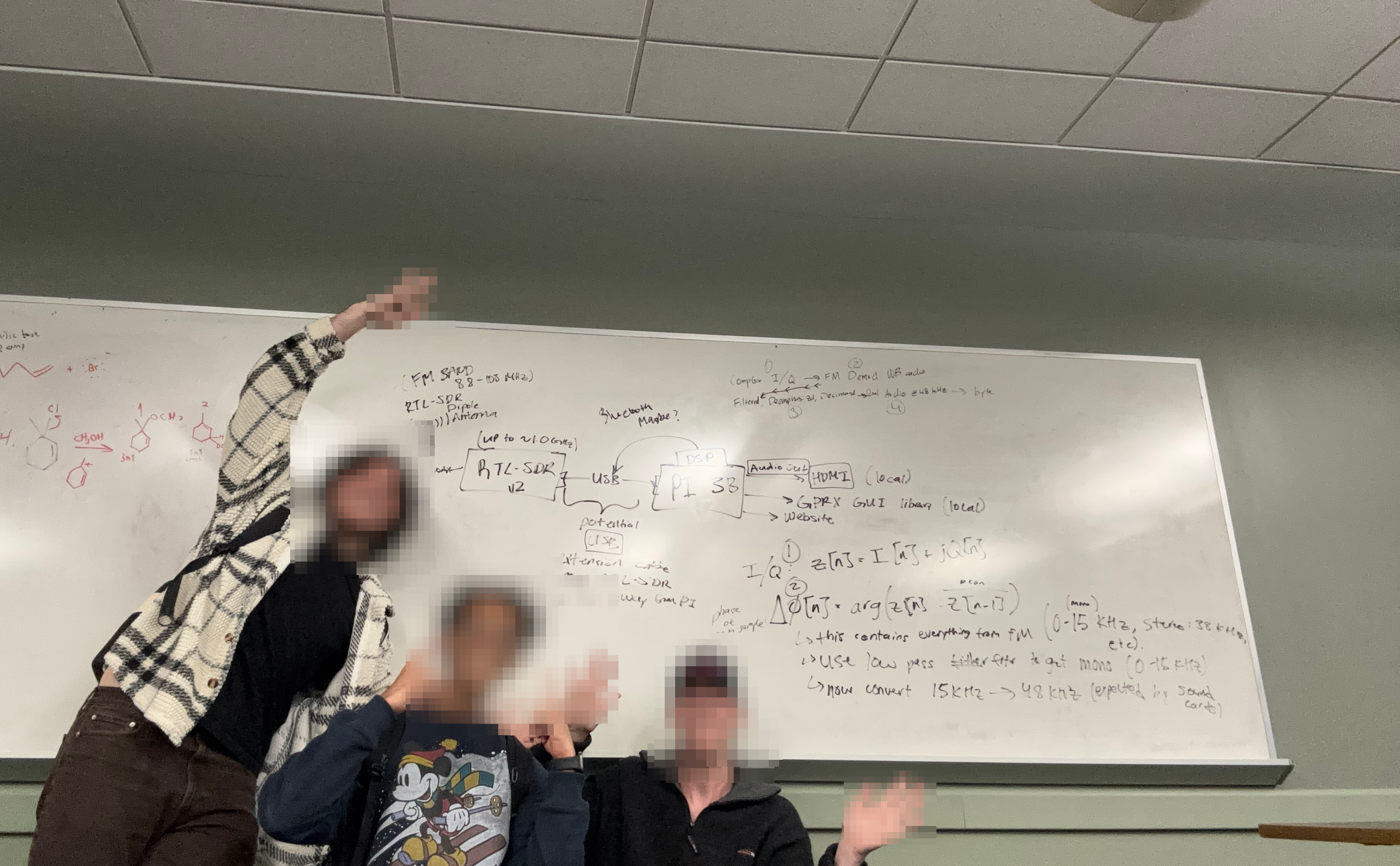
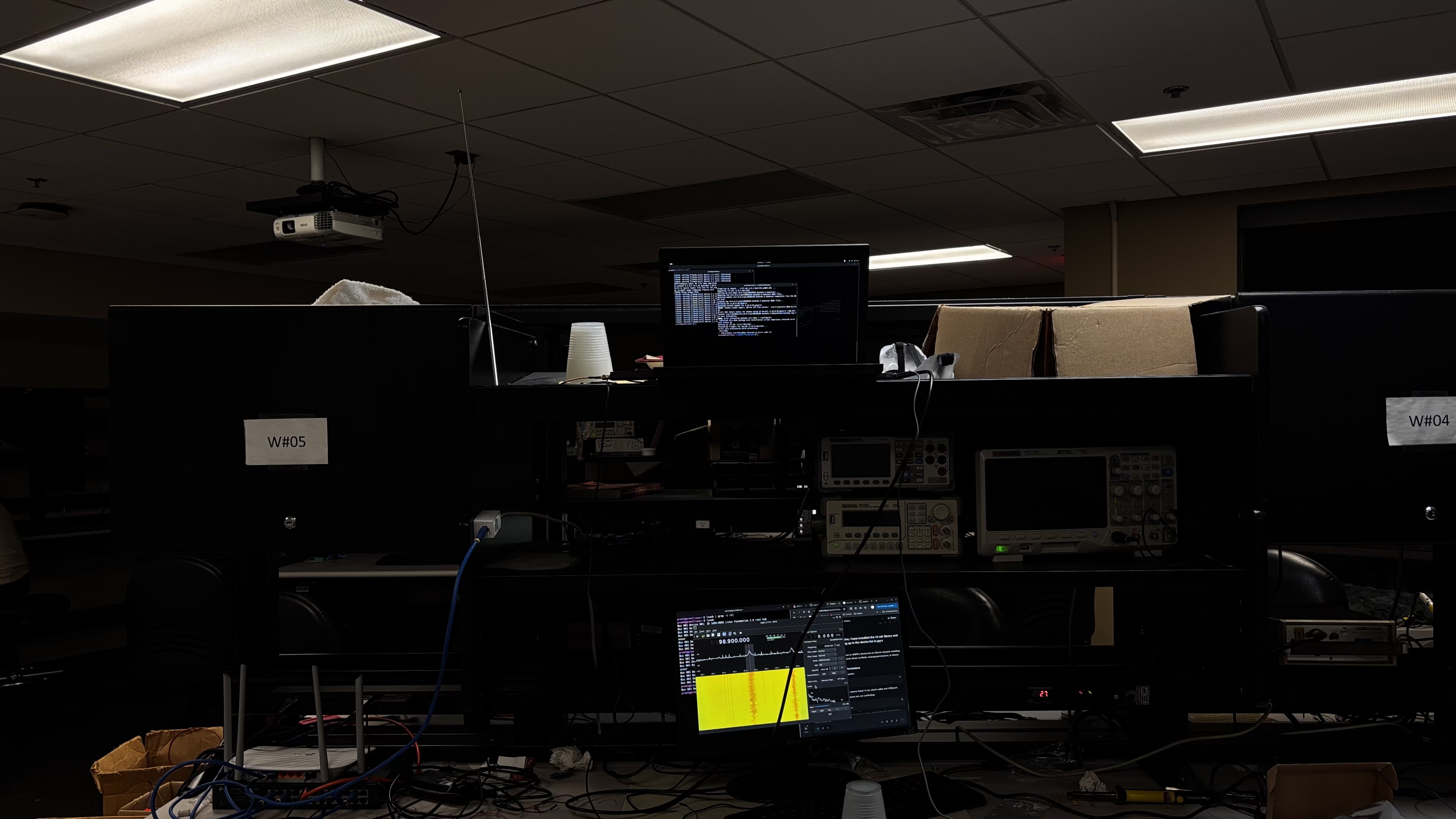
lab setup

the physics

Broadcast FM can we written as:

s(t) = A_{c}\cos(2\pi f_{c}t + 2\pi k_{f} \int_{-\infty}^{t}m(\tau)d \tau )

- $A_{c}:$ broadcast amplitude
- $f_{c}:$ broadcast frequency
- $m(t)$ : message audio
- $k_{f}$ : frequency deviation constant

If you take the derivate of the phase form, you get the instantaneous angular frequency

\begin{aligned} w(t) = \frac{d \theta(t)}{dt} &= \frac{d}{dt}(2\pi f_{c}t + 2\pi k_{f}\int_{-\infty}^{t}m(\tau)d \tau ) \\ &= 2\pi f_{c} + 2\pi k_{f}m(t) \end{aligned}

so the audio m(t) is literally hiding in the rate of the change of the phase

The RTL-SDR and its analog front end downconvert and sample this into complex basebound:

z[n] = I[n] +jQ[n] \approx A[n]e^{j \phi[n]}

Two consecutive samples:

z[n] = Ae^{j\phi [n]}, \;\; z[n-1] = Ae^{j\phi[n-1]}

and multiply by the complex conjugate:

z[n]\overline{z[n-1]} = (Ae^{j\phi [n]}) \;(Ae^{j\phi[n-1]}) = A^2e^{-j(\phi[n]-\phi[n-1])} = A^2e^{j\Delta\phi}

So now:

\Delta\phi[n] = \phi[n] - \phi[n-1] = \text{arg}(z[n]\overline{z[n-1]})

where $\text{arg}(z)$ is the 2D polar angle in radians, $\varphi$ , from the real axis to vector $z$ ( $\varphi \gt 0$ if measured counterclockwise), or algebraically defined:

z = r(\cos\varphi + i \sin\varphi) = re^{i\varphi}, r = \lvert{z}\rvert = \sqrt{x^2 + y^2}

basically, the phase difference is the difference the angles of two samples

But why multiply by the complex conjugate?? This is the digital demodulation trick!
Instead of calculating the phase of every single sample using $\arctan(Q/I)$ and then dealing with phase wrapping (where the angle jumps from $\pi$ to $-\pi$ ) which is very computationally expensive.

bridging the gap

So once you're satisfiyed with "FM audio just being phase change", turning this into code is suprising short. We first focused on getting a static implementation down, using I/Q sample data from GQRX

load the complex I/Q
channel low-pass around the FM station ( $\pm$ 80 kHz)
FM demodulation (get the phase difference)
decimate down to audio-friendly rates
de-emphasis with $\tau$ = 75 $\mu s$
write 48 kHz WAV

# static_demod.py
import numpy as np
from scipy.signal import firwin, lfilter, decimate
from scipy.io.wavfile import write
 
samples = np.fromfile("gqrx_..._2048000_fc.raw", np.complex64)
fs = 2_048_000
 
gain_db = -16.9
gain_linear = 10 ** (gain_db / 20)
iq = samples * gain_linear
 
cutoff_hz = 80_000
nyq = fs / 2
channel_fir = firwin(101, cutoff_hz / nyq)
iq_filt = lfilter(channel_fir, 1.0, iq)
 
v = iq_filt[1:] * np.conj(iq_filt[:-1])
fm_wide = np.angle(v).astype(np.float32)
 
fm_48k = decimate(fm_wide, q=fs // 48_000, ftype='iir')
 
tau = 75e-6
alpha = 1 / (1 + 1 / (2 * np.pi * tau * 48_000))
deemph = np.zeros_like(fm_48k)
deemph[0] = fm_48k[0]
for i in range(1, len(fm_48k)):
    deemph[i] = alpha * fm_48k[i] + (1 - alpha) * deemph[i-1]
 
deemph /= np.max(np.abs(deemph) + 1e-12)
write("static_demod.wav", 48_000, deemph.astype(np.float32))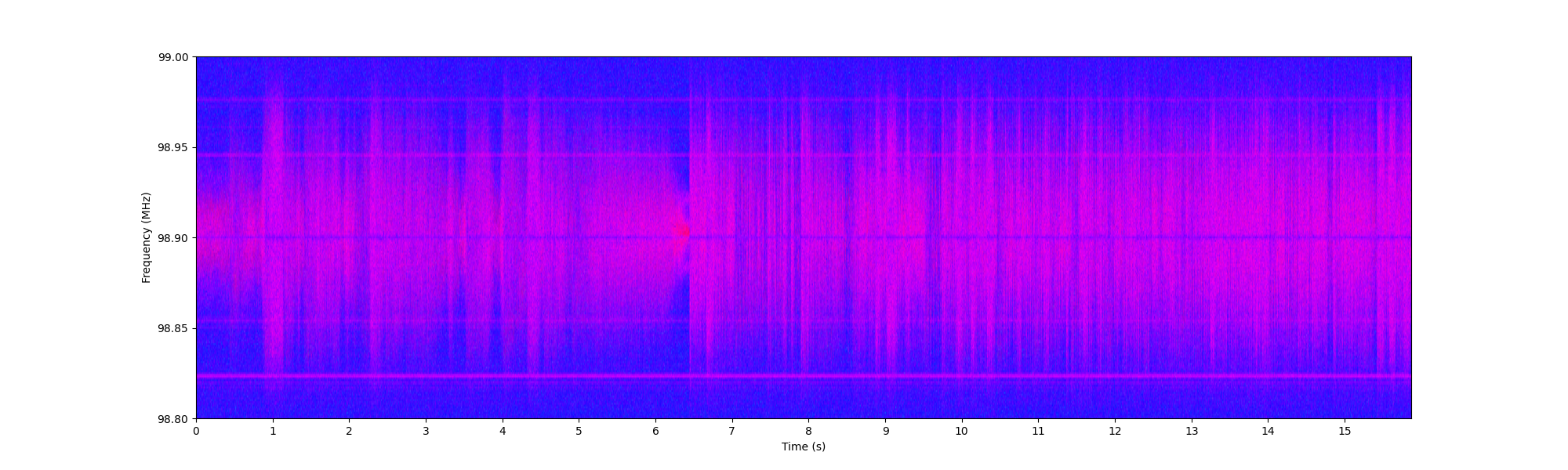

spectrogram — Figure 1. Spectrogram of 98.9 MHz FM Signal

real-time demodulation

Once the static pipeline sounded good, we upgraded it into a streaming system.

We wrapped the DSP state in a 'DSPState' class:

class DSPState:
    def __init__(self):
        self.chan_zi = np.zeros(len(channel_fir)-1, dtype=np.complex64)
        self.last_iq = None
        self.fm_buffer = np.zeros(0, dtype=np.float32)
        self.deemph_state = 0.0
 
state = DSPState()

Each incoming chunk: - complex FIR channel filter with preserved 'zi' - FM demodulation iwith continuity using 'state.last_iq' - accumulate into a buffer - soft AGC + write to output stream

The Pi could reliably pull I/Q, but doing all of this and audio on the Pi speakers was rough. On laptops, though, the dynamic demod ran smoothly with continuous FM playback; we even compared it to the station’s web stream and were beating it by 1–3 minutes (yay, lower latency than the “official” stream).

and here is the part everyone has been waiting for ... "does it even work?"

real-time demodulation of an FM broadcast signal.

~
~
<EOF>